
At the most basic level, making money from betting requires two things. Skill and luck. Whilst many bettors fail to acknowledge the influence of the latter, measuring the former is also often overlooked. This article shows why it is important to understand the different methods of assessing betting skill and how results can differ depending on your approach.
- How can bettors asses their level of skill?
- The difference between a Bayesian and frequentist approach?
- What about degrees of randomness and expected skill probabilities?
Bayes’ Theorem can be used by sports bettors to make better predictions. We can also use it to help us determine what the likelihood of us actually being any good at making those predictions and finding positive expected value. I’ve previously investigated how to evaluate the quality of a betting history using a frequentist approach (t-test). This article will compare and contrast the two methods.
Degrees of belief
In probability theory Bayes’ Theorem describes the chances of an event happening conditional on another event occurring also. For example, suppose I believe that I have a 50% probability of being a skilled bettor capable of finding value. If I win my next bet, how will this influence my belief in this proposition? In other words, how does the evidence of winning a bet change the probability of me being a skilled bettor?
Bayes’ Theorem interprets probability as a ‘degree of belief’ in a proposition or hypothesis, and formalises mathematically the relationship between the prior degree of belief before the evidence is known (the prior probability) and the degree of belief after accounting for the evidence (the posterior probability). It is written as follows:
{equation} – P(A|B)= P(A)*P(B|A)/P(B)
In our example here:
P(A) = the prior probability that I am a skilled bettor
P(B) = the prior probability of winning my bet
P(B|A) = the probability I win my bet conditional on me being a skilled bettor.
P(A|B) = the probability I am a skilled bettor conditional on me winning my bet.
Let’s try an example. Let’s assume that the definition of a skilled bettor is someone who can consistently achieve a return on investment of 110%. For even-money wagers that would imply 55 winners out of every 100. Hence, P(B|A), the probability I win my bet conditional on me being a skilled bettor, is 55%.
For an unskilled bettor, the probability of winning a fair even-money wager, P(B), will be 50%. However, let’s assume I hold a prior belief that I have a 50-50 chance of being skilled {P(A) = 50%}, and P(B) for such a bettor is 52.5% (half way between 50% and 55%).
Should I win my bet, imputing these numbers into Bayes’ Theorem yields a posterior probability – P(A|B) – of 52.38%. Winning my bet leads me to believe there is a greater probability than before that I am skilled.
Bayes’ Theorem can be applied iteratively. Having won my first bet and updated my probability of being a skilled bettor, I now place another bet. The posterior probability calculated in the first step becomes the new prior probability.
The new posterior probability of me being a skilled bettor will now be conditional on me winning (or losing) my next bet. If I win, the probability of me being skilled will increase again; if I lose, it will decrease. In this example, should I win my second bet, the probability that I am a skilled bettor increases to 54.75%.
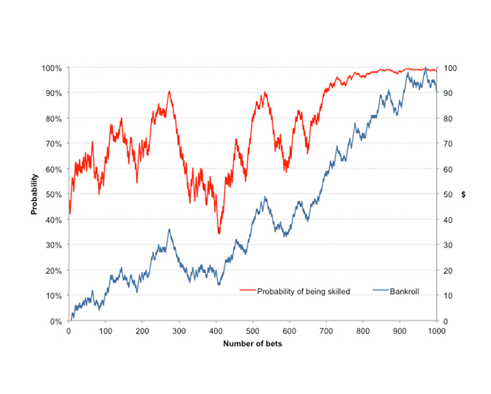
This process can be repeated indefinitely with each updated conditional probability falling somewhere between 0% and 100%. I have run this iteration 1,000 times, i.e. 1,000 wagers, and the chart below shows the betting history achieved (blue line) alongside the Bayesian probabilities of me being a skilled bettor after each wager (red line).
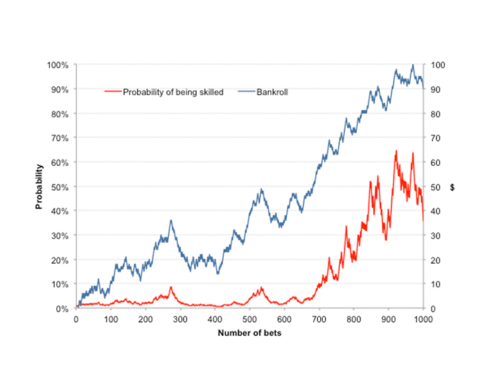
One significant problem with a Bayesian interpretation of probability is that it requires strong prior knowledge or belief in an event or situation. But do we really have that in assessing the probability that I might be skilled at betting? My choice of 50% in this example was purely arbitrary and based on nothing else than guesswork. Look what happens if I now change the initial prior probability to 1%.
Furthermore, it is completely arbitrary what skilled actually means in this context. Arguably a bettor capable of 105% return on investment is highly skilled if he can achieve that over 10,000 wagers – you can read about the Law of Small Numbers to find out why sample size matters. It’s also equally unclear how to define P(B) for each iterative step, given an updated value of P(A).
In my Bayesian model, I simply assumed a linear relationship, such that if P(A) = 0%/20%/40%/60%/80%/100%, then P(B) = 50%/51%/52%/53%/54%/55%, but its validity is certainly open to question. Perhaps more importantly, since an individual with a baseline bet win probability of 52.5% is clearly a skilled bettor in his own right (just not as skilled as one with 55%) really what we are measuring here is the degree, rather than the probability, of skill.
Nonetheless, this graphical representation of the evolution of Bayesian probability does provide some intuitive measure of the likelihood (or strength) of the ability of a bettor to return a consistent profit, and how that might change over time.
Degrees of randomness
Whilst the Bayesian approach focuses on the probability of a hypothesis (that I am a skilled bettor) given a fixed set of data (the profits and losses), the frequentist approach focuses on the probability (or frequency) of the data given the hypothesis. This time the hypothesis is fixed – it’s either true (100% probability) or false (0% probability) that I am skilled – whilst the data are assumed to be random.
Typically, the frequentist approach starts with the null hypothesis, in this case I am not skilled and that my betting outcomes are all a consequence of luck. It then attempts to calculate the probability (usually called the p-value) by means of some statistic that the data we have observed, in this case my history of profits and losses, could have happened assuming the null hypothesis to be true.
Finally, that probability is compared to an acceptable significance value (sometimes called the α-value) such that, if p < α (typically 5% or 1%), the null hypothesis is rejected in favour of the valid one.
The statistic that I have reviewed previously on Pinnacle’s Betting Resources is the t-score, so named as it is derived from the student’s t-test for statistical significance. Assuming that betting odds are fair, the t-score can be approximated by:
where n = the number of wagers, r = the return on investment (expressed as a decimal) and o = the average decimal betting odds. The t-score is converted into a p-value by means of statistical tables or an online calculator. In Excel, one can use the TDIST function. Let’s look at how this plays out with our example betting history.
The chart below compares the original time series of evolving Bayesian probability – that I am a skilled bettor with an original prior belief of 50% probability that I am (red line) – with the evolution of the frequentist p-value – the probability that what I have achieved could have happened by chance assuming I have no skill at all (green line), using a two-tailed, one-sample t-test.
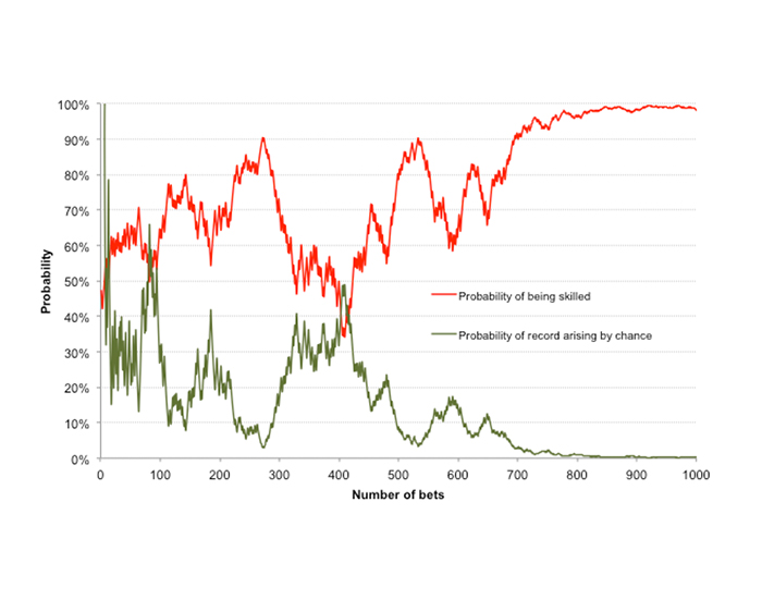
In a generally qualitative way the two lines are mirror opposites, although this is more likely a result of good fortune than anything else. One should not, however, take away the message that the p-value measures the probability of being unskilled, and that 1-p therefore is equal to the probability of being skilled.
A probability of 5% that our history of profits and losses has occurred by chance is not the same thing as a probability of 95% that they are occurring because of skill. It simply means that assuming the null hypothesis – that wins and losses in betting are purely random – is true, what we have observed could be expected to occur 5% of the time.
The weakness of the frequentist approach is that it treats truth as an absolute. In contrast, the Bayesian approach implicitly considers truth to be probabilistic, provisional and always falsifiable. Despite this shortcoming frequentist hypothesis testing nonetheless offers us an equally useful tool with which to analyse a history of betting, and to ascertain whether it is likely to have arisen through something other than good fortune.
How do the frequentist and Bayesian models compare if the latter has an original prior belief of just 1% probability (rather than 50%) that I am skilled?
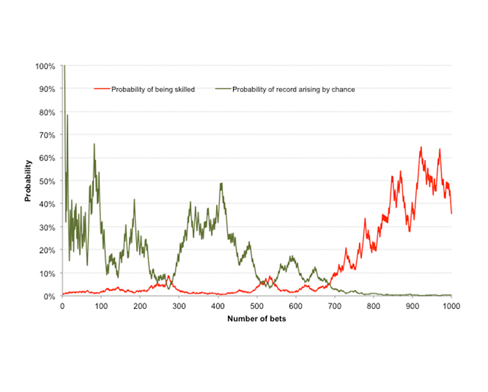
This time it is clear that our t-test will be encouraging us to believe much more readily in our ability as a skilled tipster than the Bayesian approach, which by contrast is much more conservative.
This further highlights the sensitivity of Bayesian probability to an initial prior belief. In this case, after nearly 700 bets, whilst our t-test might tell us our betting history has just a 3% probability of occurring by chance, Bayes’ Theorem would imply there’s still less than a 10% chance of us being skilled enough to deliver a 110% return on investment over the long term.
Being the risk-averse bettor that I am, my preference would be for the more conservative prior belief in ability: unless I have good reason to doubt it, I should always begin by assuming that I have little or no skill whatsoever.
Expected skill probabilities
The analysis above presents just one random example of a betting time series with a hypothesised 110% return on investment. In the interests of visual clarity I deliberately picked a betting history that allowed me to convey the ideas discussed.
To get a more detailed picture of expectation, however, that is to say what we should expect to see on average, we should run the model many times. Those of you familiar to Pinnacle’s Betting Resources will know we can do this via means of a Monte Carlo simulation.
The first chart below shows the results of a 10,000-run Monte Carlo simulation of the evolution of the Bayesian probability that I am a skilled bettor for ten hypothesised win rates: 51% through to 60% at 1% intervals (equivalent to 102% to 120% expected value at 2% intervals assuming fair odds).
The curves have been constructed by calculating the median value of Bayesian probability after each sequential wager during the 1,000-wager history, which for this purpose offers a better representation than the mean (where low and high values can skew the interpretation).
The initial prior belief in my skill {p(A)} is assumed to be 1%. Unsurprisingly, the higher my hypothesised win rate (and expected value), the faster the belief in my ability approaches 100% probability. (The darker the curve the higher the hypothesised win rate.)
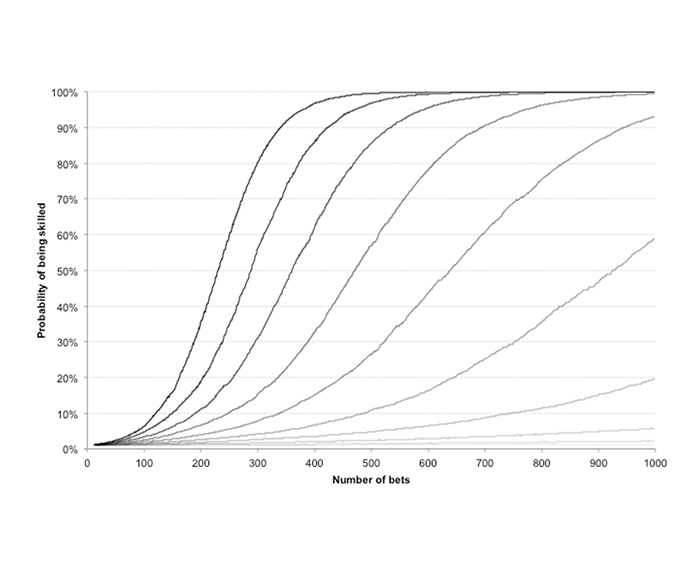
The best handicappers in the business are typically capable of about 57% win rates. After the bookmaker’s margin, that translates into about a 110% return on investment. This chart illustrates that if you are aspiring to become one, it is going to take the best part of 1,000 wagers to acquire a strong and meaningful belief in your abilities, assuming of course you initially believed that you had little ability to begin with.
By contrast, if you find yourself winning a lower 54% of your spreads, whilst still profitable, it will take a lot longer than that to have real faith in what you are doing. Starting from a prior belief of 1% probability that one is skilled, this will have risen to just 20% after 1,000 wagers.
The final chart shows a similar set of idealised expected p-values from the same 1,000-wager history and same ten hypothesised win rates. Since we have an equation for approximating the t-score for any combination of bet number, return on investment and betting odds, a Monte Carlo simulation is not required. Again, the darker the curves the greater the hypothesised win rate (from 51% through to 60%).
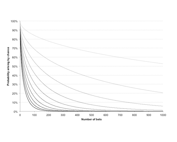
With a win rate of 57%, statistical significance (p-value < 5%) is achieved after just 200 wagers, with stronger statistical significance (p-value < 1%) coming after about 335 wagers. To reiterate, however, this information tells us nothing about our levels of betting skill, simply the likelihood of this history arising by chance, assuming no skill at all.
Additionally, these levels of statistical significance, like the initial Bayesian prior probabilities, are based on little more than subjective judgement. But like the Bayesian model, p-value statistical testing should, if bearing these caveats in mind, offer a useful method of helping the bettor assess their abilities at finding a consistently profitable expectation.
If nothing else, both Bayesian and frequentist analysis should further serve to remind the bettor that betting for consistent profit is a long game. Never assume that a few wins imply that you know what you’re doing.
About the author