The model simulations discussed so far are based on one major assumption: closing odds are completely independent of opening odds, that is to say they have no memory. We know that in a time series of bets, each outcome has no memory of the last, there is no such thing as a hot streak, and the gambler’s fallacy is an expression of those who fail to recognise this truism. However, the relationship between opening and closing odds is arguably a different ball game (pun intended).

Let’s suppose instead that when a price longer than the ‘true’ price is published, it is more likely that it will close still longer than the ‘true’price. Conversely, when a shorter than ‘true’ price is published it is more likely to close still shorter than ‘true’.

Why should this be the case? Well, since the ‘true’ price remains unknown, both to the bookmaker and their customers, the actual value of the opener could be hypothesised to act as a kind of anchor or reference point which biases judgement and restricts the magnitude of future movements. Sure, pricing mistakes will be exploited, but possibly not by as much as they should be. That, at least, is the idea.

Price anchoring and random variability will provide counter balancing forces on the extent to which the opening/closing price movement can be used to predict a bettor’s expected profits.

Anchoring is a cognitive bias familiar to behavioural psychologists. In a betting context the price a bookmaker offers publicly may have the potential to subconsciously influence how a bettor views a match. The view that they form may very well be different to the view they might have formed had they studied the match before seeing the bookmaker’s price.

The majority of bettors will probably look at the odds before deciding whether to bet rather than undertaking their own analysis to determine a ‘true’ outcome probability. Thus, when a bettor sees a bookmaker’s price of 2.25, they might take the view that the ‘true’ price is 2.05, and not 2.00. The act of observing the 2.25 may influence their judgement to the extent that they will deviate away from the ‘true’ price and towards the anchor price. A similar argument can be applied to prices shorter than ‘true’.

Testing the influence of anchoring on odds movement

For the purpose of my model, instead of using 2.00 as the expected closing price, a value was chosen for each bet that was anchored to the opening price. Different anchoring strengths were tested, from just 10% (an opening price of 2.20 would have an anchored closing price of 2.02) up to 90% (2.20 and 2.18). Again, those anchored closing prices were varied randomly using a range of standard deviations (0.15 down to 0).

Thus, a price opening longer than ‘true’ could still close shorter than ‘true’ due to inherent random variability, but the anchoring ensured that any closing deviation shorter than ‘true’ would on average be smaller than the original deviation longer than ‘true’. Since the opposite is true for opening prices shorter than ‘true’, the average closing price for the sample of 10,000 bets is still 2.00, and hence still collectively efficient.

I’ve illustrated the effects of anchoring closing prices by 20% in the three charts below for three different random closing price variability (σ = 0.09, 0.06 and 0.03). Compare these to the equivalent charts above without anchoring.

This time, the ‘Coefficient of Proportionally’ between the Opening/Closing price Ratio (minus 1) and profitability (or Yield) (or OCRYCOP as I referred to it in part one of this article) is the value of the gradient of the trend line. A value of 1 implies perfect proportionality OCRYCOP values are higher (0.73 versus 0.81, 0.88 versus 1.00 and 0.96 versus 1.17). Indeed in the final chart OCRYCOP is actually greater than 1, with profits still available at closing prices for the biggest opening/closing price ratios. Essentially, because of the anchoring influence, opening prices longer than 2.00 still contained some expected value at closing. The converse is true for shorter than ‘true’ prices.

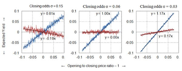
The middle chart above offers a model scenario – 20% price anchoring and σ = 0.06 for random closing price variability – that looks a lot like Pinnacle’s real data. We’ve managed to achieve it without needing perfect price efficiency at the level of individual betting odds. Intuitively this makes more sense.

As mentioned, it would seem highly improbable that every Pinnacle closing price was perfectly accurate. It also gives succour to those who support the idea that you don’t necessarily need to always beat the closing price to be a sharp bettor.

At the level of individual bets there will be occasions where a closing price is not perfectly ‘true’ and hence you will not need to beat it to hold profitable expected value. Of course you still always need to beat the ‘true’ price, whatever that may be.

The charts above present just three model scenarios. There are many other possible combinations of anchor strength and random closing price variability. I tested 54 of them. The OCRYCOP figures are tabulated below. Recall that figures more the 1 imply that on average opening prices longer than ‘true’ will still hold some value by closing, whilst figures less than 1 imply that on average opening prices longer than ‘true’ will have shortened too much.

Evidently, where there is too much inherent random variability in closing prices about the ‘true’ price (σ = 0.09 and higher), it is impossible to generate a model scenario that replicates Pinnacle’s data. The opening/closing price ratio will always underestimate the expected profit over turnover (OCRYCOP < 1), regardless of any price anchoring.

Essentially this implies there is an upper limit to the amount of random variation in closing prices about ‘true’ prices for OCRYCOP to be a useful predictor of profitability. In fact that limit occurred at σ = 0.075 with a 50% price anchoring (in other words about half the standard deviation in the opening odds).

As the table above illustrates there is more than one way to create a model scenario with OCRYCOP = 1. Difference combinations of price anchoring and random closing price variability will work. The final table shows model scenarios capable of generating OCRYCOP figures ≃ 1 along with the standard deviations in the opening/closing price ratios.

σ = 0.06 for closing price variability, for example, offers two opportunities for matching Pinnacle’s data. We’ve already seem a price anchoring of 20% does the job. But so too does an anchoring of 80%. Is such a figure realistic? Probably not, since it implies that bettors on average would be heavily biased by a publication of a price, even where those prices contain significant errors. It would also imply far less price movement than actually occurs in practice.

The majority of bettors will probably look at the odds before deciding whether to bet rather than undertaking their own analysis to determine a ‘true’ outcome probability.

The standard deviation in opening/closing price ratios in the full Pinnacle data set is 0.103, and 0.082 for a restricted set of opening odds between 1.5 and 2.5. In contrast the standard deviation for the model scenario with 80% price anchoring and σ = 0.06 for random closing price variability was just 0.033, compared to 0.068 for 20% price anchoring. The lower anchoring seems much a better fit with real world data and intuition.

Possibly an even better pairing would be 10% anchoring and σ = 0.045, if we subscribe to the idea that sharper bettors in a Pinnacle betting market won’t typically be suffering from anchoring bias as much as more recreational bettors at a recreational bookmaker. Anchoring = 5% and closing price σ = 0.033 works too, as does 2% and 0.02 and 1% and 0.015, but now we are almost back to perfect price efficiency on an individual bet basis and that seems unrealistic.

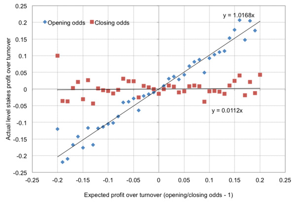
Is there any evidence for price anchoring? Well, unless Pinnacle’s closing prices are pretty close to being perfectly efficient individually, there really is no way to generate an OCRYCOP figure of 1 without it. You might now very well make the point that whilst my model was focused around odds of 2.00, the Pinnacle data contained odds across the full spectrum of outcome probabilities. That is indeed true; so here is the OCRYCOP chart for the restricted odds range 1.50 to 2.50 (a total of 109,619 betting odds).

Furthermore, I’ve had a look at some data from a collection of recreational bookmakers available via a leading odds comparison service. A sample of 30,540 average betting odds had an OCRYCOP figure of 1.51. Admittedly the sample is much smaller than the Pinnacle data I analysed but the evidence of residual market inefficiency at closing is compelling.

Remember, OCRYCOP > 1 implies odds longer than they should be relative to ‘true’ don’t shorten (or steam) enough before closing, whilst odds shorter than they should be don’t lengthen (or drift) enough before closing. I’ve previously written about the evidence for steamers not steaming enough and drifters not drifters not drifting enough.

Recreational bookmakers with less sophisticated customers more prone to anchoring bias may arguably exhibit OCRYCOP figures considerably greater than 1. Conceivably, however, those recreational bookmakers may also prefer to hold attractive prices longer than ‘true’ rather than allow traditional market forces to have free rein, presumably for advertising purposes. That, too, would deliver the same result.

There is one final point I should address. Even the model scenarios with the most opening/closing price ratio variability show less variability than the real world data. The highest figure of σ = 0.0749 occurs, unsurprisingly, for perfect individual odds efficiency and no price anchoring. That compares to 0.082 for data in the chart above.

Broadly speaking they are similar, but introducing price anchoring reduces the ranges of opening/closing price ratios. Can we account for the difference? Possibly; if we take out Pinnacle’s most extreme opening/closing price ratios (where the odds have moved the most), the value of σ is reduced. Removing only the most extreme 1% lowers the figure to 0.770.

Arguably some of those extreme price movements may represent palpable errors on the part of the data source recording Pinnacle’s opening and closing betting odds. Additionally, some extreme movements will arise on account of extreme changes in information about the teams in question which are beyond the ranges of random distribution in a model. On account of both reasons, the real world data is likely to have fatter tails in the distribution of price movements, and hence greater variability, than my simple model would imply.

What have we learnt?

Pinnacle is the standard bearer of betting price efficiency. Its closing prices offer a reasonable way of estimating your expected profitability. Nevertheless, my investigation has shown that the efficiency underlying their betting market is more nuanced than it would first appear.

On average, Pinnacle’s closing prices closely reflect the ‘true’ probabilities of things happening. Individually, however, this need not be the case. Price anchoring and random variability will provide counter balancing forces on the extent to which the opening/closing price movement can be used to predict a bettor’s expected profits.

The implication of what has been uncovered is that bettors don’t always need to beat a closing price to believe they are still sharp, since price anchoring will preserve some residual inefficiency even at market closure. At Pinnacle, it is probable that both price anchoring to an opening price and inherent random variability of closing prices about ‘true’ prices is small. However, we have now seen that we don’t necessarily need every price to be perfectly efficient to build a market that is collectively very accurate, and how that can happen in practice.