Understanding the strengths and weaknesses of the model

In part one of this article I explained an approach for modelling momentum between sets in a tennis match using serve percentages. In doing so, it was shown that updating serve percentage expectations only at the end of each set wasn’t dynamic enough. For this reason, the model was limited in that it couldn’t price totals and handicaps.

Now, in part two, I will discuss an update to the model that better reflects momentum both within and between sets during a tennis match.

In part one, I showed that a player is more likely, on average, to win the second set if they have won the first. The first step in building a more dynamic model is understanding how the margin of victory in the first set is related to the winner of, and margin of victory, in the second set.

Measuring momentum from the first set to the second

The chart below plots the first set winner’s margin of victory (in games in set one) against their set two win %. For example, players with match winner implied probabilities 71-80% who win the first set by five or six games, (6-1 or 6-0), win the second set 83% of the time.

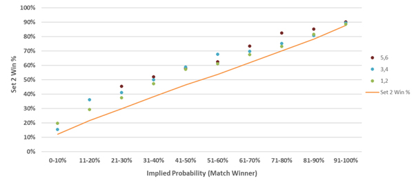
There appears to be definite positive relationship between the margin of victory in the first set and the outcome of the second. The relationship does break down for big underdogs (<20% implied probability), although there were significantly fewer matches in this range. We can unpack this result a step further, and compare the margin of victory in set one with the margin of victory in set two.

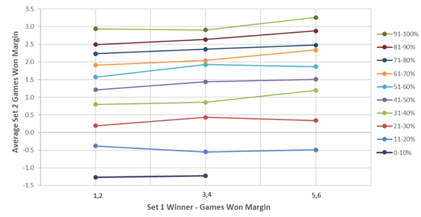
Again, a momentum effect is observed. A larger margin of victory in set one leads to a larger margin of victory in set two, on average. With these results, I updated the average service percentage change required for set two, in an identical way to what was shown in part one of this article.

So we now know the magnitude of set two serve percentage updates required after set one, (knowing the margin of victory) however we want to update these more dynamically – after each game, or ideally after each point. The next step is determining which incremental updates to make during the set.

I propose modifying player serve percentages after each game to reflect set by set momentum. My calculation for these updates uses both the score (incorporating the number of breaks of serve) and the players’ observed serve percentages.

The predictive power of these two variables will overlap somewhat. However in some cases, one may offer a signal when the other doesn’t. For example, in an even money match, if we compare scores of 3-3, and 4-2, the players’ serve percentages may be identical in both, yet the player leading 4-2 will be more likely to win the set (and thus the next set also). Similarly, at 3-3, there could be a difference in serve percentages, despite the even scoreline.

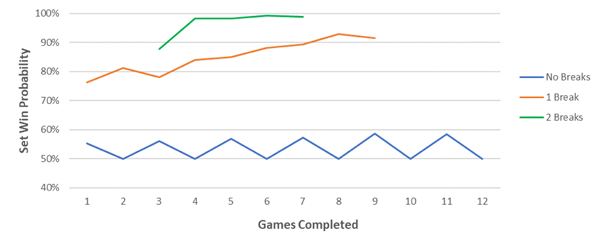
To determine the proportion of serve percentage updates to be applied after each game, I use the likelihood of winning the set for each player, estimated from 30,000 simulations. The chart below plots this for an even money match. For example, after six games, if there is one service break (a score of 4-2), the player leading is expected to win the set with a probability of 88%. My model allocates that player 88% of the applicable serve percentage adjustment at that point of the match.

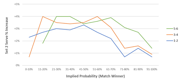
The adjustments are also scaled based on observed relative serve strength after each game. Relative serve strength is the difference between Player 1 and Player 2’s observed serve percentages.

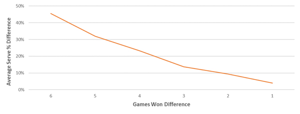
To determine the relationship (and thus the magnitude of scaling required) between serve percentages and set scores, I simulated 30,000 matches and calculated the difference in serve percentages for different scores. For example, for completed sets with a difference of two games (6-4 or 7-5), the average difference in serve percentage was +9% to the winner.

Using the above calculations to apportion serve percentage updates dynamically after each game throughout a match, we can now simulate our model and compare it to actual outcomes in ATP matches. The chart below plots 30,000 simulations of the model against all ATP matches since 2010 in the (match winner) implied probability range 40-60%.

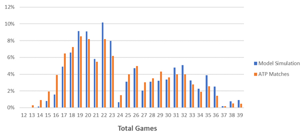
The model appears improved from the initial one shown in part one of this article. However, it still underestimates game totals of 18 or less. This suggests that the model still needs to be quicker in adjusting to one-sided matches.

Due to tennis’ set-based scoring, a player behind a break or two in a set may lose interest and/or save energy and concentration for the next set. To reflect this (as well as short term momentum more generally), I suspect that I need to include a ‘within set’ momentum factor to complement the ‘between sets’ updates above.

Without game-by-game data, I landed on the magnitude of this factor through simulations. What I learned was that the model needed to adjust very rapidly to ‘within set’ performance.

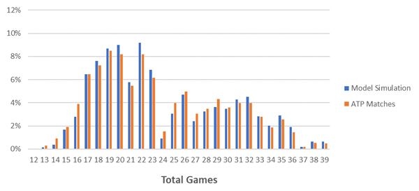
The magnitude of the serve percentage updates required was almost double that of the ‘between sets’ variable. Simulating the model a further 30,000 times, we can see that the addition of a ‘within set’ momentum factor increases its accuracy.

Serve percentage and match totals betting

We can now use this model to price match totals. First, let’s see how a total games market would change in an even money match as we alter the serve percentages. In the table below I simulated 10,000 matches for each serve percentage and framed a no margin market.

As the players’ starting serve percentage increases from 50% to 72%, the total games line increases from 19.5 to 25.5.

With serve percentages over 72%, at least 26 games (two tie break sets) becomes the favourite. To put this in context, the players with the highest serve percentage in the ATP top 50 are Isner and Federer who both win around 72% of points on serve.

There are only a few matchups in the ATP that would justify a match total of 25.5. The match up would be between two evenly-favoured big servers with poor returning. What happens to these markets if instead of an even money match, there is a 1.50 favourite?

Serve percentage and handicaps betting

Next let’s consider match handicaps. Varying the favourite and underdog’s serve percentages around the ATP average serve percentage of 64%, we can investigate how the match odds relate to the game handicap line.

Cross checking these with Pinnacle’s tennis markets, we can see that the model is calibrated quite well. In order to price individual matches, the final step would be forecasting individual player serve percentages and adjusting for player specific biases. This may include adjusting the momentum factors to reflect a certain player’s patterns. I discussed a number of these in another previous article.

The result of including two dynamic momentum variables to my ATP tennis model is a well-calibrated model that can now be used to price game, set, match, total and handicap markets from serve percentages.

An additional step may be to include score-specific and/or player biases. For example, when serving under pressure to stay in a set at say *4-5 or *5-6, is a player less likely to hold serve? With a few additions such as this, the model could easily be extended to be an in-play one.