In February 2019, Pinnacle’s Betting Resources published my article modelling a bettor’s range of possible betting returns. Around an expected performance there is a distribution of possible outcomes influenced by good and bad luck, defined by the mathematics of the normal distribution. To help bettors visualise this, I made available a simple performance distribution calculator.

This analysis only considered stakes of the same size (level stakes). Whilst I’m very much an advocate of this money management strategy, others quite reasonably prefer a different one. The most common one is to bet a percentage stake based on the current size of one’s bankroll.

Unsurprisingly, the aforementioned method is known as percentage staking. It’s a strategy I’ve discussed before on Pinnacle in comparison to level staking. The simplest version is to bet the same percentage for every bet, regardless of the odds. More sophisticated versions, like Kelly staking, advocate taking both the odds and the size of one’s expected value into account when defining the percentage size.

How does percentage staking work?

Suppose a bettor starts with a bankroll of 100 units. They decide they want to bet 1% of their bankroll on their bets. The first bet will therefore be 1 unit. If it wins at odds of 2.00, the bankroll will now stand at 101. Hence, their next bet will have a stake of 1.01 units, which is 1% of 101. If the first bet had lost, the bankroll would stand at 99 units and the next bet would have a stake of 0.99 units.

Kelly staking specifically defines the percentage figure that should be applied by dividing the expected value by the decimal odds minus 1. For example, a bet at odds of 3.00 with an expected value of 10% or 0.1 would be assigned a percentage stake of 0.1 / 3 – 1 = 5%. There are those who argue Kelly staking is too risky to be considered a realistic money management strategy, since it can sometimes advise very large percentage figures. To moderate this risk, fractional Kelly is often considered.

The skewed distribution of possible returns from percentage staking

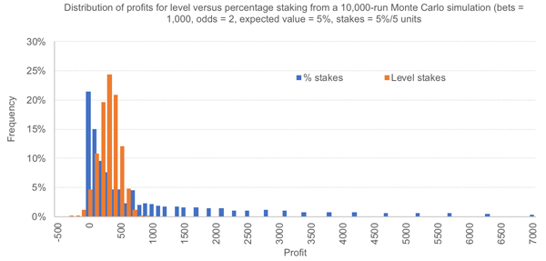
The chart below (reproduced from my earlier article on Pinnacle) compares the distribution of possible returns for level stakes versus percentage staking for one betting scenario produced via a Monte Carlo simulation. In comparison to level staking, percentage staking, with some good fortune, can see some very big bankrolls.

The distribution has what we would term positive skew. In this scenario, some profits were considerable larger than 7,000 units but for clarity I have omitted them.

Quantifying returns mathematically

In fact, for the simplest of scenarios where the odds and stake percentage of every bet are the same, we don’t need to resort to a Monte Carlo simulation; it’s possible to produce the distribution mathematically.

Consider the following example. A bettor places their first bet at evens with a 10% stake. If it wins, their bankroll is now 110% (or 1.1) times the original bankroll. If it loses, it will be only 90% (or 0.9) times the original bankroll. The same is true after each sequential bet. Consequently, if the bettor bets 10 times and has six winners, we can easily calculate the growth in their bankroll as follows:

Bankroll growth = 1.1⁶ x 0.9⁴ = 1.162 or 116.2%

It doesn’t matter what order the wins and losses come in. The bettor could start with six winners and finish with four losers; or they could start with four winners and finish with six losers; or any other of the 210 total possible ways of arranging this combination of winners and losers. They will still finish with 116.2% of what they started with.

Thus, for n bets with stakes S% and w winners:

Bankroll growth = (1 + S)^w(1 – S)^n-w

The biggest bankroll growth in my Monte Carlo simulation above was 948.8. I haven’t kept the actual win/loss figures but knowing there were 1,000 bets with odds of 2.0 and stakes of 5%, I can use this formula to determine that the actual number of winners was 581.

Furthermore, if we know the expected value (EV) for our bets, we can calculate the expected rate of bankroll growth as follows:

Expected bankroll growth = {(EV x S) +1}ⁿ

For example, if this bettor’s EV is 20% or 0.2, their expected (or mean) bankroll growth will be given by {(0.2*0.1)+1}¹⁰ = 1.02¹⁰ = 1.219 or 121.9%. Readers might observe that this is greater than the bankroll growth associated with winning six out of 10 even-money bets, which is what is implied by a 20% EV.

This is because the bankroll growth for more wins contributes disproportionately more to the average than those for fewer wins – remember the distribution of possible returns is positively skewed. Thus, whilst the most typical (median) bankroll growth in this example will be 116.2%, the expected (or mean) value will be 121.9%.

Obviously, this assumes that EV is the same for every bet, a huge oversimplification but necessary to define the mathematics.

If we rewrite (EV x S) + 1 as the expected bank growth factor, F, then we have:

Expected bankroll growth = Fⁿ

,and thus:

n = Log_F(Expected bankroll growth)

,where F is the base of the logarithm.

For bets with the same stake percentage and EV, the logarithm of the expected bankroll growth will be proportional to the number of bets. Similarly, the logarithm of the actual bankroll growth will also be proportional to the number wins. This is visually demonstrated for our example bettor here. The second chart is the same as the first but with a logarithmic y-axis.

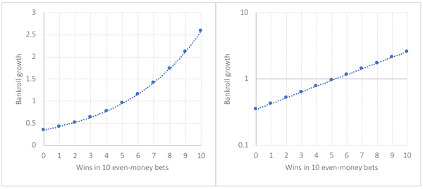
You may have noticed that five wins and five losses, which for a level staker would result in a break-even return from even-money bets, results in a slight loss with percentage staking (bankroll growth = 0.951). It takes a bigger percentage growth to recover a previous loss, but if percentages for stakes stay the same, one win following one loss won’t quite recover the initial lost stake. Similarly, one loss following one win will lose you more than you initially won on your first bet. The same is true over 10 bets (or any number of bets). If the bankroll growth for one win and one loss is 0.99 (1.1 x 0.9), then for five wins and five losses it is 0.99⁵ = 0.951.

The skewed distribution of returns from percentage staking is log-normal.

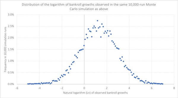
If the number of wins in a series of bets is proportional to the logarithm of the bankroll growth, we should expect to see a log-normal distribution of possible bankroll growth.

A log-normal distribution is one where the logarithm of the data is normally distributed (the familiar bell-shaped curve). Below I have plotted the frequency distribution of the natural logarithm (Ln) of the 10,000 observed bankroll growths from the same Monte Carlo simulation I referred to earlier.

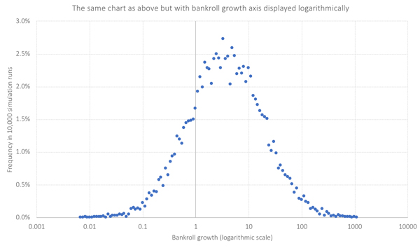
Instead of transforming the bankroll growth figures logarithmically, I can instead display the original figures using a logarithmic scale. The results are visually equivalent.

The average or expected bankroll growth for this Monte Carlo sample was 12.2. How does that compare to the figure calculated from first principles using the equation above? With an EV of 5% (0.05) for the 1,000 bets and the stake size 5% (or 0.05), the answer is 1.0025¹⁰⁰⁰ = 12.1, an excellent match. Unsurprisingly, the median bankroll growth (the centre of the distribution) was considerably lower at 3.49, with only 21.7% of bankroll growth figures higher than the expected figure of 12.2. Remember, a few very large bankrolls positively skew the mean.

Estimating the probability of bankroll growth

Is there a way to calculate the probability of achieving a specific bankroll growth? One can look at the chart above and make visual estimates, although given the logarithmic scale, that is no easy task. Alternatively, we can just count the number of times a bankroll finished higher than a certain threshold. In this Monte Carlo sample, for example, a bankroll finished with more than it started with (bankroll growth = 1) 78.5% of the time, and at least doubled 63.5% of the time.

However, using Excel there is an easier method. Having calculated the natural logarithm (using the =Ln function) for all simulated bankroll growth figures, it is then possible to use the follow function:

1 – LOGNORM.DIST(x,mean,SD,true)

where x is your chosen bankroll growth threshold value (for example 2 for a doubling), ‘mean’ and ‘SD’ are the average and standard deviation respectively of your natural logarithm values, and ‘true’ ensures a cumulative probability. Using this formula, the probability of finishing with more than you had started with (x = 1) was estimated to be 78.2%, the probability of doubling your bankroll (x = 2) was 63.6% and the probability of exceeding expectation (x = 12.2) was 21.7%, almost the same figures as from counting.

A percentage staking bankroll calculator

Provided all our bets have the same odds and stake percentage, we can build a calculator to put our bankroll growth equation to work, plotting the distribution of possible bankroll growth figures for different win/loss rates. Using an Excel calculator that I have built for my own website, the charts below show outputs for various betting scenarios.

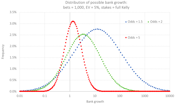
The first compares the performances of three different betting odds using a fully Kelly staking plan over 1,000 bets. With bets holding an EV of 5%, the percentages stakes for odds 1.5, 2.0, and 5.0 respectively are 10%, 5% and 1.25%. Expected bankroll growth for these three odds scenarios are 147, 12.1 and 1.87, whilst median bankroll growth figures are 12.7, 3.49 and 1.36. The green distribution is effectively a match for the Monte Carlo distribution above, given that the inputs for the model were the same.

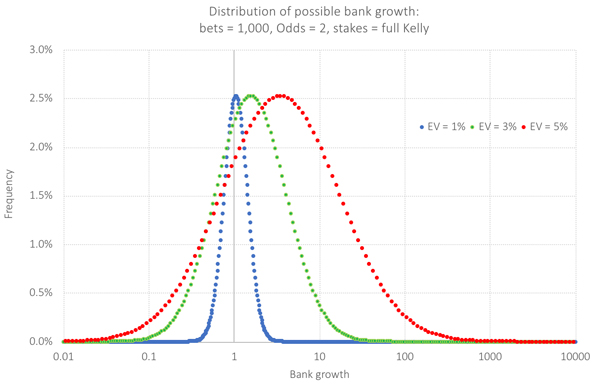
The next chart shows how the bank growth distribution varies with EV. Three scenarios are shown: 1%, 3% and 5%, all with odds of 2.0 and 1,000 bets and again with a full Kelly stake (1%, 3% and 5% respectively). Expected and median bankroll growth for these were 1.11, 2.46 and 12.1, and 1.05, 1.57 and 3.49.

The third chart illustrates how the bankroll growth distribution changes when we reduce the size of the Kelly fraction. With odds of 2.0 and EV of 5%, full, half and quarter Kelly stakes are 5%, 2.5% and 1.25% respectively. Expected and median bankroll growth for these were 12.1, 3.49 and 1.87 and 3.49, 2.55 and 1.73.

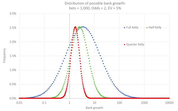
As mentioned earlier, fractional Kelly is often advocated to moderate risks. The distribution above illustrates why. Whilst the probability of poor performance is reduced significantly (compare the area to the left of bank growth = 1 for the blue and green distributions), the median bankroll is only marginally smaller (2.55 compared to 3.49).

Granted, your expected (mean) bankroll growth is much bigger with full Kelly but most of the time you won’t see that. The median is arguably a better measure of what you should expect to happen in this context. With full Kelly you still have a 21.5% chance of making a loss. For half Kelly, that reduces to 11.8%.

Expected and median bankroll growth

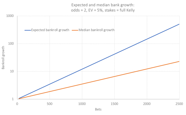
We can use the calculator to see how the expected bankroll growth will vary with the number of bets. We already know from our equations above that this will be logarithmic. The median bankroll growth also varies logarithmically.

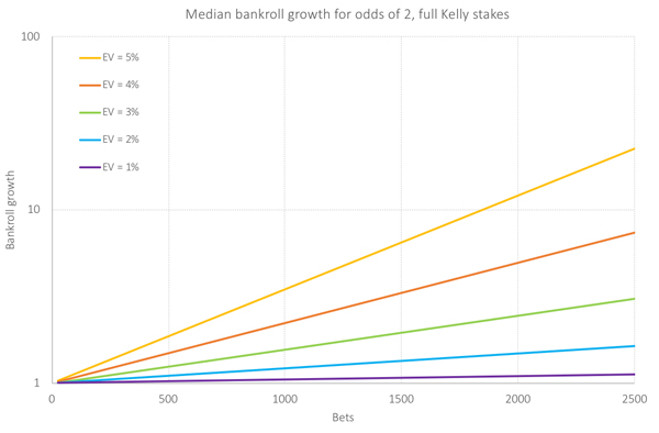
Finally, see how the median bankroll growth varies with your EV. Again, this scenario is for odds of 2.0, but you could create similar charts for other betting odds.

Variable odds, variable stakes

The equations and calculator described relying on all bets having the same odds and same stake percentage. How robust will they be under real world scenarios where both may vary? Testing against Monte Carlo simulations reveals that odds can vary considerably without having too much impact on the reliability of the calculator’s outputs, but only provided the stake percentages are all the same. Obviously, that will not be the case with Kelly staking.

The calculator is also robust for variable stake percentages, for example those advised by the Kelly strategy, provided the odds don’t vary too much. A typical example would be Asian Handicap or point spreads, where most odds are close to 1.95, with minimal deviation.

Reliability is weaker when EV for these bet types also varies, but again provided neither the odds nor the EV for those bets varies too much, the calculator offers a reasonable method of providing quick estimates of performance expectation.

We know that defining expectations from level staking is relatively straight forward. However, this article has shown that we can do the same for percentage staking too. Whilst level staking performances will be normally distributed, those from percentage staking are distributed log-normally. Using this information, I have been able to develop a simple calculator to help bettors define their range of expectations should they choose to follow this money management strategy.