In a recent twitter discussion, I reviewed the returns of a well-known racing twitter tipster. From 1,015 daily naps (their best rated tips for the day) their profit over turnover to level stakes was -4.3%.

“That’s a decent sample to test their overall profitability,”

I remarked, without giving it too much thought. A thousand tips, after all, is a pretty decent size, isn’t it? To be sure, only last month I was discussing again how randomness can influence outcomes over samples as large as this.

Nevertheless, aren’t we on reasonably solid ground believing this tells us the tipster in question is probably not giving us the “best quality horse racing tips on the internet” as was being claimed?

One of my twitter followers took issue; “not that I disagree with your point… But are 1,000 bets enough to conclude anything?”

After a moment’s reflection, I decided they’re probably not. I issued a response.

“Actually, you have a point. The average odds of the winning naps are 2.62. Let’s suppose the other two-thirds that are losers (for which odds were not shown) had slightly longer odds (that’s why they lost), making the overall about 3.00.

The expected standard deviation in yield for a sample of 1,015 bets would be about 0.045 (4.5%). Suppose their long-term expectation is -4.5%. They would then be close to it. Instead suppose their expectation was break even. They’d be about one standard deviation away from it – unlucky, but well within the realms of natural variation.

Now, instead suppose they should be doing +4.5%. That’s about two standard deviations away from where they are, or about 2.5% probability. They could still just about claim that their long-term expectation was +4.5% but that they had been unlucky. For still higher expected returns, however, it becomes harder and harder to argue that what they’ve done in 1,015 bets is just bad luck.”

How did I come up with a figure of 4.5% for an expected standard deviation in the yield? The purpose of this article is to explain exactly that, as well as how it can help us judge our actual betting performance against any expectations me might have.

The mathematics of betting returns distributions

Bets are binary propositions: they either win or they lose. In November 2018 I reviewed how the binomial distribution can be used to inform us about the possible distribution of wins and losses for a sample of bets that are subject to the vagaries of randomness. For a sample of n bets where each one has a ‘true’ win probability p, the standard deviation, or spread, of possible sample win percentages is given by the following formula:

For example, if we have 100 bets and each has a 50% probability of winning, we should expect to win 50% and the standard deviation will be 5%. In other words, about two-thirds of all possible outcomes will fall between 45% and 55%, with about 95% of them falling between 40% and 60%.

Never mind wins and losses, what about actual profits? We just need a little adjustment to the formula above, by including the betting odds. Now, where each bet has odds o, the standard deviation in possible yields (or profit over turnover) is given by:

Suppose in this example our ‘true’ win probability was 60% for even-money odds offered by the bookmaker, a very generous coin toss indeed. The standard deviation in possible yields from 100 wagers would be 9.798% or about an expected yield of 20%.

For fair odds, o = 1/p, the formula above reduces to:

Although this special case only really applies where a bettor has break even expectation (yield = 0%), the difference between o and 1/p is typically small, whether for unskilled bettors suffering the bookmaker’s margin, or skilled bettors who have managed to overcome it, so one might justifiably use it for simplicity. This is illustrated in the figure below.

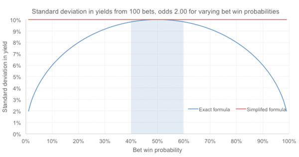
For this example, using this short-cut formula would always give us a standard deviation of 10%, no matter what the value of p. But that’s pretty close to the actual standard deviation for win probabilities between 40% and 60%. No bettor, at least with Pinnacle, should face win a percentage as low as 40% for even-money propositions.

Most Pinnacle margins are of the order of 1 to 3%; odds of 2.00 with a 2% margin imply a win probability of about 49%. (The actual 100-bet yield standard deviation would be 9.998%.) Similarly, the world’s best handicappers show win percentages around 55% to 56%. (The 100-bet yield standard deviation would be 9.928%.)

What can the yield standard deviation tell us?

Let’s go back to the example I introduced at the start to reveal what information the yield standard deviation can give us. Assuming an average bet price (o) of 3.00 for the 1,015 level stakes wagers (n) and a ‘true’ win probability of 32% (p) implied by an expectation of -4.3%, our equation above gives us a yield standard deviation of 4.39% (or 4.44% using the short cut formula).

The distribution of possible betting yields around the expectation will look like the one drawn below. You can draw these easily yourself in Excel simply using the NORMDIST function. Although in theory these distributions are binomial and therefore discrete, at samples above about 30, the (continuous) normal distribution is a very reliable approximation and lends itself more readily to drawing these charts in Excel.

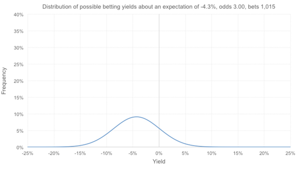
The area under the blue curve will add up to 100%. In this scenario we have assumed that the actual yield is matching expectation. However, because the odds are quite long, there is a fairly wide spread of possible outcomes, ensuring that even the mostly likely outcome, the -4.3%, will happen less than 10% of the time.

Was that Twitter follower right to question my initial observation? Arguably, I think he was. Whilst it’s clearly not a record representative of the best quality horse racing advice, it’s not at all obvious that the advisory service holds negative expected value. 13.65% of possible yields in this scenario are profitable, well within boundaries of statistical acceptability. Perhaps the tipster holds a better expectation than -4.3% and they’ve just been unlucky.

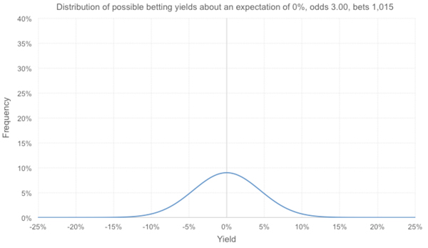
Suppose instead, as I argued in the introduction, the tipster’s expectation was break even. Now the distribution would look like this: 16.13% of yields in this scenario are less than the actual performance, far too high to rule out the possibility that it’s been unlucky.

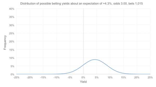
What if the expectation was +4.3%? Now we have the following distribution. There are still 2.76% of outcomes that perform worse than the actual record. That’s small but can we really decide to rule out bad luck completely? That’s more than 1 in 40 tipsters, and in for example 4,000 tipsters it’s going to happen.

Finally, let’s suppose this tipster were to claim that they really did offer the best racing advice on the internet and that more commonly they would be showing a 10% profit over turnover. Their possible yields would be distributed as follows.

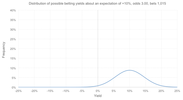
Nearly 2% of them are unprofitable, but fewer than 1-in-1,000 are worse than the observed 4.3%. Arguably it would now be time to call out this tipster for a case of overconfidence bias.

If we know our average odds, our yield and our number of bets, we can calculate our expected standard deviation in possible yields and plot pretty much any distribution we want. As I have done here, it’s possible to contrast what we’ve actually achieved against a range of opinions about what we think we might be capable of achieving.

Where there’s only a small chance that our actual yield can happen, given our opinion about what we think should be happening (say less than 1% or even 0.1%), we should consider evaluating our expectations.

Changing the betting odds

How does the distribution in possible betting yields vary for different betting odds? Take a look below; these are for scenarios where the expectation is to break even.

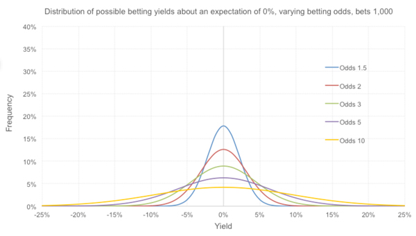
Unsurprisingly, the longer the odds the greater the variance or spread in outcomes. Of course, for these expected break-even scenarios the variance (or square of the standard deviation) is directly proportional to the odds minus 1.

Betting at longer odds will mean you have a greater chance of doing a lot better than expected just because of good luck (the distribution tails are fatter at higher yields). Of course, the reverse, is unfortunately also true since the distributions are symmetrical.

Changing the length of the betting history

We can also see how the size of the betting history influences our distribution. The formula above informs us that the yield standard deviation is inversely proportional to the square root of the number of bets. Hence, a break-even expectation from 100 even-money bets (10%) will have 10 times the spread for an equivalent record of 10,000 bets (1%). Some others are illustrated below.

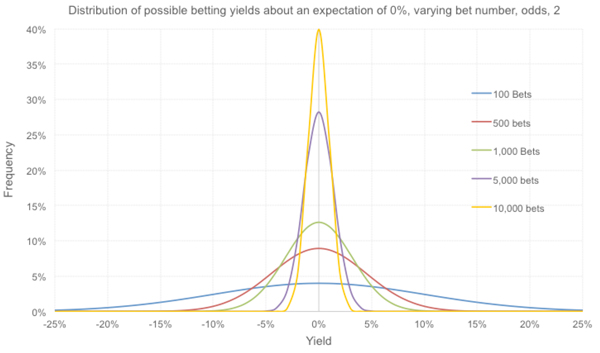
The narrowing of the distributions with increasing length of betting history, and their increase in height, is essentially a visual interpretation of the law of large numbers. The larger our sample the more likely it is that what we’ve achieved is a measure of our real expected value.

How long can unskilled betting careers last?

As a final thought experiment, consider how long it might take an unskilled Pinnacle handicapper with an expectation of -2.5% to realise that they are unskilled. Knowing one’s expected yield standard deviation can offer some clues.

The table below shows the probability that the handicapper will still be showing a profit after a series of bets for different betting odds.

With small margin bookmakers, a little bit of luck can take you a long way, particularly for longer odds. Of course, if you’re unlucky, longer odds will be a much faster route to bankruptcy.

Here’s a similar table, but this time for the probability of showing losses of 10%. This is simply a consequence of their greater variances (and wider distributions of possible yields).

How robust is the formula with real world betting histories?

Lastly, you might well be wondering how robust my formula is for estimating the yield standard deviation when betting a range of odds. Thus far, I’ve simple assumed all bets have the same odds. Of course, most bettors bet all sorts of prices. Can we just take an average value for the betting odds and get a reliable figure for the yield standard deviation?

With small margin bookmakers, a little bit of luck can take you a long way, particularly for longer odds. If you’re unlucky, longer odds will be a much faster route to bankruptcy.

Returning to the tipster’s record at the start of this article, I’ve artificially filled in the missing odds (for the losing tips that were never published) to make the average odds 3.00. My actual spread of odds was considerable, from shortest prices of 8/11 (1.73) up to 14/1 (15.0).

Using Excel’s random number generator to simulate results where the expectation for every bet is -4.3%, I ran a 100,000-iteration Monte Carlo simulation, giving me 100,000 different yields for the sample of 1,015 bets. The average yield was -4.297% and the standard deviation in those yields was 4.373%. Within acceptable margins of error, that’s effectively the same as the value predicted by my formula, 4.389%.

Some of you may have noticed the similarity between this methodology and my t-test method for estimating the likelihood that a betting record could arise by chance. Essentially the two methods are very similar in approach. Indeed, at even modest sample sizes (n > 30), the binomial, normal and t-distributions are essentially the same thing.

Hopefully, this article offers a better visualisation of the different ranges of expectation a bettor has depending on their preferences and performances.

In addition to my existing t-test calculator for testing a betting record, I have now also made available a yield distribution calculator which you can use to test your own records.