Pinnacle’s Head of Trading Marco Blume has made it clear that a reliable indicator of whether a bettor holds long term profitable expected value – that is to say they are sharp – is whether they can beat the closing line.

It is commonly assumed that a market’s closing price is the most efficient, or accurate, of all betting prices, reflecting as it does the most amount of information available about a game. If, after the influence of the margin, it reflects the ‘true’ probability of something happening, then any amount you beat it by will be a measure of the expected advantage you hold.

Beat it by 10% and you can expect to make a 10% profit over the long run. There are others, however, who have argued that whilst beating the closing line is an important sign of skill, it is not necessarily a prerequisite. For that to work, however, it implies that closing prices cannot always be fully efficient.

In this article I want to attempt to reconcile these two positions, looking again at the concept of efficiency and in particular the efficiency of Pinnacle’s closing prices as a means of arriving at a consensus. I’ll say now that the read might not be for the faint-hearted, being a journey into my statistical thought experiment.

When I embarked on it I wasn’t sure what I would find. Even at the end I still remain unsure about the conclusions, but stay with me. It might not be as fun a trip through Willy Wonka’s chocolate factory, but hopefully it will be more enlightening for those aspiring to be sharp bettors.

What is market efficiency?

Over the past few years I’ve talked quite a lot about the concept of market efficiency. In a betting context, an efficient market is one where the betting odds accurately reflect the underlying outcome probabilities of the events in question. For example, if the ‘true’ probability of Manchester City inflicting humiliation on their rivals Manchester United was 70%, then odds of 1.429, before the bookmaker added their margin, would be efficient.

Betting markets, after all, are pretty effective Bayesian processors, continually refining, upgrading and improving views about the probability of something happening.

Naturally for a single match, there is one or other result, and a bet on Manchester City will win or lose. However, repeated many hundreds or thousands of times, the good and bad luck of individual bets on individual games will cancel out (the law of large numbers). Hence, it is still meaningful to talk of the ‘true’ probability of a result, even though in practice it is impossible to know precisely. That, after all, is what the betting odds are a reflection of.

Market efficiency is an interesting concept applied to large samples. However, for single events if we can’t really know what the ‘true’ probability of an outcome actually is, how can we ever know how efficient the betting price was?

Sure, we can test a large sample of bets, say, with fair odds (no margin) of 2.00. If 50% of them win that tells us that in aggregate the average win probability of those bets was probably 50% and hence on average the odds of those bets were a reasonable reflection of their underlying win probabilities. But it tells us nothing about the individual win probabilities of those bets that contributed to the overall average. A market might be collectively efficient but masking underlying efficiencies on a bet-by-bet basis.

How efficient are Pinnacle’s closing odds?

In July 2016 Pinnacle published my article that revealed how efficient (or accurate) their soccer match betting odds are, and in particular their closing odds, the final published prices before a match starts.

Once their margin is removed, I showed that odds of 2.00 win about 50% of the time, odds of 3.00 win 33% of the time, odds of 4.00 win 25% of the time, and so on. Of course, as explained earlier, none of that told us anything about the ‘true’ outcome probabilities of individual matches, just that on average, the odds were pretty accurate.

More than this, I showed how the ratio of Pinnacle’s opening to closing price was a very reliable indicator of profitability, implying their closing odds were highly efficient. For example, teams that opened at 2.20 (with the margin removed) and shortened to 2.00 by closing won about 50% of the time and returned a level stakes profit over turnover of 10% to the opening price (or 2.20/2.00 – 1) and 0% to closing prices.

On the other hand, teams that opened at 1.80 and then drifted to 2.00 won about 50% of the time and showed a 10% loss to the opening price (or 1.80/2.00 – 1) and 0% to closing prices. I’ve run the analysis again with an increased sample size of 158,092 matches and 474,278 home/draw/away betting odds and the results and conclusions are broadly the same. They are illustrated in the chart below.

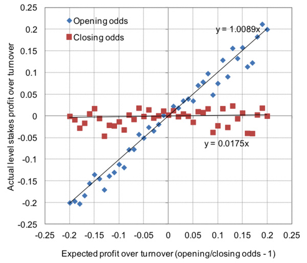
Each data point represents the actual returns from 1% intervals of the opening/closing price ratio. Points in blue are the returns from the opening prices, points in red the returns from closing prices. Evidently there is some underlying variability, but the generalised trends are clear. I’ve shown the trend lines, opting to set their intercepts at zero (arguably a reasonable assumption where the margin has been removed), and their equations.

They confirm again my original hypothesis almost perfectly, that the opening to closing price ratio (x on the chart) is an excellent predictor of profitability to opening prices (y on the chart), and more generally that, on average, Pinnacle’s closing prices are highly efficient.

The ‘Coefficient of Proportionally’ between the Opening/Closing price Ratio (minus 1) and profitability (or Yield) is the value of the gradient of the trend line. A value of 1 implies perfect proportionality. For brevity I will abbreviate this coefficient with the acronym OCRYCOP for the remainder of this article.

Again, however, we still only know this to be ‘true’ in aggregate. We’re still none the wiser about how efficient individual closing odds actually are. Each data point in the chart had thousands of contributing matches.

Modelling market efficiency

In an attempt to uncover how we might arrive at such an OCRYCOP chart that implies closing price efficiency I built a simple model simulating opening to closing price movements. The model consisted of 10,000 bets, each with an opening and closing price.

In attempt to replicate the uncertainty about the bets’ ‘true’ outcome probabilities, I decided to randomise the opening odds around an average of 2.00 with a standard deviation (σ) of 0.15 (implying about two-thirds fell between 1.85 and 2.15 and 95% fell between 1.70 and 2.30).

Thus, whilst the ‘true’ price for every bet, known only to Laplace’s Demon (and me), was 2.00, the opening price published by my hypothetical bookmaker in my model varied somewhat about that average. I chose the figure of 0.15 for the standard deviation since it broadly it reflects observed opening to closing price movements in real betting markets where odds are close to 2.00.

A standard deviation of 0.05, for example, would imply that 95% of published opening odds of around 2.00 would be accurate to within ±5%. That seems too narrow a range, given the amount that prices are actually observed to move. Similarly a figure of 0.3 or higher would suggest the bookmakers aren’t very good at setting odds, something we know generally not to be ‘true’.

Market efficiency is an interesting concept applied to large samples. However, for single events if we can’t really know what the ‘true’ probability of an outcome actually is, how can we ever know how efficient the betting price was?

It’s highly unlikely that a bookmaker would ever set a price of 3.00 for a ‘true’ price of 2.00. Yes, it can happen, but that’s usually a palpable error or the consequence of some unforeseen and significant piece of news which was unavailable at the time they set the odds. In such circumstances, of course, it’s perfectly reasonable to talk about the ‘true’ price changing too. Anyway, back to the model. I’ve made some opening odds; what about the closing ones?

Closing odds, in theory, reflect opinions expressed financially by bettors. Let’s assume that in the extreme, despite those opinions reflecting an accumulation of information about the ‘true’ outcome probability, there remains the same level of inherent random uncertainty. Obviously that doesn’t seem realistic – betting markets, after all, are pretty effective Bayesian processors, continually refining, upgrading and improving views about the probability of something happening, thereby reducing the level of uncertainty about that.

In terms of our model, the average price and standard deviation are again respectively 2.00 and 0.15. For each opening and closing odds pair we can now calculate a ratio (opening/closing). And for each, knowing the ‘true’ outcome probability (50%), we can calculate expected returns for both opening and closing odds for all 10,000 matches. Finally we can chart how expected returns from both opening and closing prices vary with varying opening/closing price ratio, just as I did for the Pinnacle match odds earlier.

The first of the six charts below shows the model results. The blue and red lines show the 50-match running average expected profit over turnover to level stakes (y-axis) to opening and closing odds respectively, having ordered the 10,000 bets by opening/closing odds -1 (x-axis). It doesn’t look much like the Pinnacle data above.

Although in aggregate both my opening and closing prices are theoretically efficient, since on average they both match the ‘true’ prices, in fact the opening/closing odds ratio predicts only half the expected profit (OCRYCOP = 0.5). For example, a ratio of 110% gives a return of 105% (or 5% profit over turnover) when bet to opening prices, and a return of 95% (or 5% loss over turnover) when bet to closing prices.

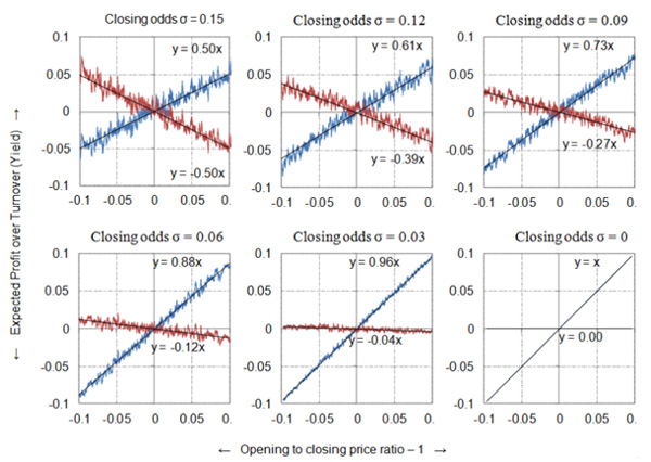
Evidently, our opening/closing price ratio in this instance is not a very good predictor of profitability, and by extension, our closing prices, individually, can’t be very efficient. The reason, of course, is simple. Firstly, we know that our closing prices are not individually efficient – they aren’t all the same as the ‘true’ price of 2.00, since I intentionally varied them randomly about that figure.

Secondly, the biggest opening/closing price ratios will occur when my random odds generator outputs a long opening odds and a short closing price. The biggest ratio generated here was 1.55 (with opening odds of 2.27 and closing odds of 1.46). Really, for opening odds of 2.27 where the ‘true’ price is 2.00, our expected profit will be 2.27/2.00 – 1 = 0.135 or 13.5%, and not 55% as predicted by my initial hypothesis.

The additional five charts above repeat the model, but gradually decreasing the random variability (standard deviation) in my closing odds, by increments of 0.03 (whilst leaving the same variation in the opening odds). You will notice that as the variability in the closing odds about the ‘true’ price of 2.00 shrinks, so the value of OCRYCOP tends towards 1. In the extreme where all closing odds are 2.00 and hence perfectly efficient individually, there is a perfect 1:1 correlation.

Look again at the earlier chart from the real Pinnacle betting odds. The trend lines (and their equations) are a pretty close match for our model example showing perfect correlation. Yet we can see clearly that there is still underlying variability – the dots don’t all lie perfectly on the trend lines. Some of that, of course, will be due to good and bad luck in actual real world results (since my model uses expected profit, good and bad luck is eliminated).

Nevertheless, surely it is completely unrealistic to believe that every individual closing price will perfectly match the ‘true’ odds. The problem, however, is that without perfectly individually efficient closing prices, we are forced to accept a less than perfect correlation between opening/closing price ratio and expected returns (OCRYCOP < 1). Is there a way to solve that? I will address exactly that in part two of this article.