Related Articles

I’ve worked in sports modelling for the last 9 months, and there is one mathematical entity that has cropped up over and over again; the so called ‘logit’ function. The logit function takes a probability, p, and converts it to a value between -ve and +ve infinity using ln(p/(1-p)), i.e. the natural logarithm of the ratio of the probabilities of the event occurring and not occurring.
The logit function can be used as a transformation to an excellent ‘space’ within which to work with probabilities. Say you’re trying to model a tennis match, and you naively claim that you have a 10% greater chance of winning a point on your serve than on your opponent’s serve. Sounds reasonable, but what if there is a very one sided match, where the favourite is expected to win 95% of points against their serve, clearly the 10% addition no longer applies. The problem is that linear shifts don’t work well in probability space, a 1% change in probability for a p = 0.5 event is far less consequential than a 1% change for a p = 0.02 event. This is a great shame, as linear additions form the backbone of most regressions and models. Instead we can transform our probability into a space where linear additions do make sense, apply the addition then transform back to probability space.
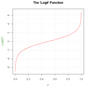
A convenient choice is ‘logit space’. Take your probability, find ln(p/(1-p)), add the shift, then use the inverse function (called the logistic function, 1/(1+e^(-x))) to return the value to a probability. As the logit function asymptotes to -ve and +ve infinity at P=0 and 1, we no longer have to worry about a shift taking us outside the viable range for probabilities, and, as you would hope, the shift causes a larger change in probability at 50% than at 2%.
Linear shifts in logit space are the mathematics behind logistic regressions. If you ever need to quantify the relationship between a ‘predictor variable’ and a probability, for instance the binary predictor variable ‘has the team received a red card’ and the probability of scoring a goal in a given minute of a football match, then logistic regressions are the way to go. My in-play basketball model relies heavily on multinomial logistic regressions. These are an extension of the logistic regression to calculate the effect of a predictor variable (or many predictor variables) on not just one, but a set of probabilities for an event with many possible outcomes. For instance, in basketball, how do the time through the match and the point difference affect the probabilities of each possible outcome of a possession, e.g. two point field goal, three point field goal, defensive rebound etc. Using the resulting regression coefficients you can create a function that ‘takes in’ values for the point difference and the time at which a possession occurs, and returns predicted probabilities for the outcome, with the logistic aspect ensuring the sum of the probabilities is always 1. I’d highly recommend using the ‘multinom’ function in R’s ‘nnet’ package. Although if you’re dealing with ‘Big Data’ of over a million samples, be prepared to set aside a couple of hours per regression.
The logit function can be used as a transformation to an excellent ‘space’ within which to work with probabilities.
Logit space is also very useful for quantifying your uncertainties in estimates of probabilities.For both bookmakers and sports traders it’s crucial to have a grasp of the accuracy of your price estimates. The ideal situation would be not just to assign a single value for the probability of an outcome, p, but to come up with a distribution, or probability density function (pdf), describing how likely you believe each value of p is to be the true value.
This opens up a plethora of new possibilities. For instance consider you want to price a snooker match. You have an initial estimate, p_A, for how likely ‘Player A’ is to win any given frame. However, what if during the match Player A is considerably outperforming your expectations; you want a system in place to update p_A accordingly. A mathematically correct way of automating this would be to use Bayesian Inference, which requires a distribution for your initial estimate for p_A, known as a ‘prior’ distribution. Typically in science, for physical measurements, the logical choice would be a normal distribution, however if this is used for p_A, you’re claiming there’s a chance p_A could be outside the range 0 to 1. Once again, logit space comes to the rescue; using a normal distribution in logit space (a logit-normal distribution) for your prior solves this issue, and leads to a narrower distribution at the extremities, as shown:
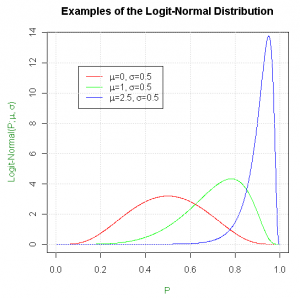
You can now quantify your uncertainty in the initial value of p_A in the value of σ for your logit-normal prior. For the more high profile matches, where you know with tighter bounds the probability of Player A winning a frame, chose a smaller value of σ. Conversely, for obscure matches, assign a larger value of σ. If Player A starts to outperform expectations, the Bayesian Inference process will result in a larger shift in the distribution for the obscure match than for the high profile match. This makes sense, as you should be more willing to revise your shaky initial estimate for the obscure match, based on the evidence provided by Player A’s performance, than your more confident estimate for the high profile match.
Now that you’ve formalised a distribution for your beliefs on the value of p_A, you can use this, as a bookmaker, in the assigning of overround to multiple selection markets (or the ‘stripping’ of overround as a trader). From my personal experience, bookmakers seem to prefer to add overround in proportion to the standard deviation of the expected frequency of an outcome, were the event to be played over and over again. However, given that you now have a distribution to describe your uncertainty, the logit-normal distribution, perhaps adding overround in proportion to a fixed shift in logit space would make more sense. At the risk of giving away too many industry secrets I’ll leave the maths up to the reader. Good luck…